
In order to learn from the beergame, the data created by the players needs to be consolidated and plotted. Here, exemplary data of one beergame session is presented.
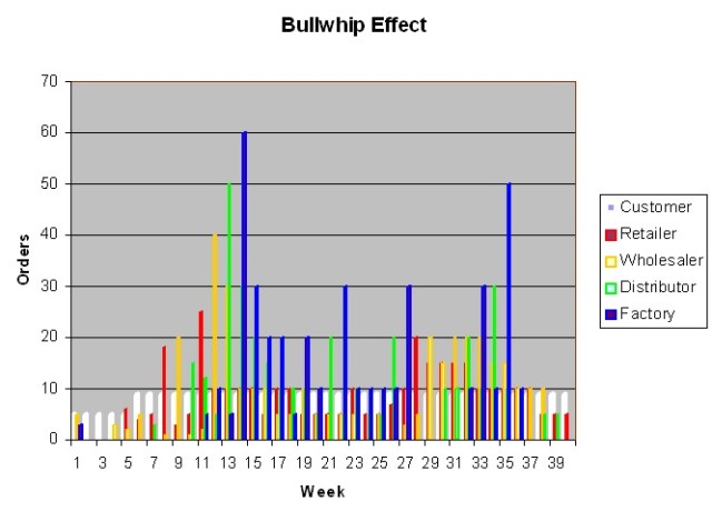
Bullwhip effect
The first figure shows the order distribution over 40 weeks and a typical bullwhip effect. It becomes obvious that the retailers reacted to the customer demand jump with a little time lag of two weeks.
Then the following stages all placed large orders, each of which magnified, thus creating a typical bullwhip effect.
Inventory fluctuation
The second figure shows the inventory fluctuation, with negative inventory representing back order.
Obviously, players move into back order. Having overreacted inventories then fill quickly in weeks 20-30.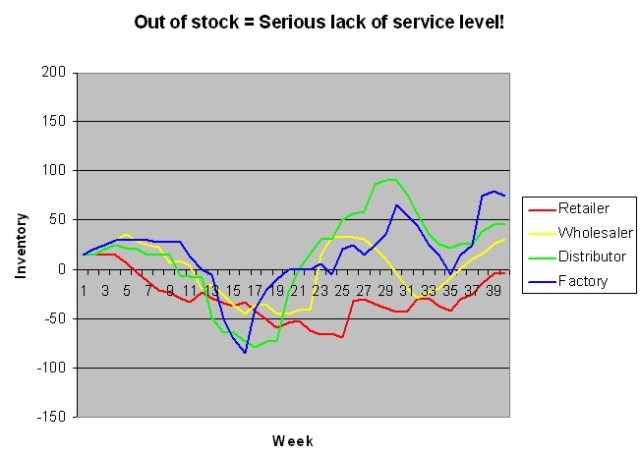
Additional data
The third figure shows some additional game data. It shows the decrease in customer demand information upstream visualised by the average order amount by the four stages. More importantly, the increase in order fluctuation upstream is illustrated by the largest amount having been ordered in each stage and the number of small orders that were placed.
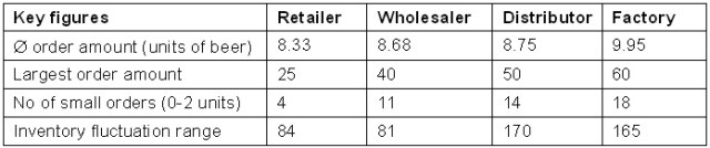
All this information is being used in the following debriefing session to discuss the bullwhip effect, its implications and the reasons for its existence.
